Spark源码学习 Join策略

学习源码所用的Spark的版本是Spark3.3.2_2.12(Scala2.12写的Spark3.3.2)

类别

Spark底层有五种join实现方式

前置介绍:HashJoin

参考资料:https://www.6aiq.com/article/1533984288407

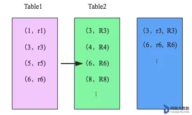
先来看看这样一条SQL语句:select * from order,item where item.id = order.i_id,很简单一个Join节点,参与join的两张表是item和order,join key分别是item.id以及order.i_id。现在假设这个Join采用的是hash join算法,整个过程会经历三步:

  1. 确定Build Table以及Probe Table:这个概念比较重要,Build Table使用join key构建Hash Table,而Probe Table使用join key进行探测,探测成功就可以join在一起。通常情况下,小表会作为Build Table,大表作为Probe Table。此事例中item为Build Table,order为Probe Table。

  2. 构建Hash Table:依次读取Build Table(item)的数据,对于每一行数据根据join key(item.id)进行hash,hash到对应的Bucket,生成hash table中的一条记录。数据缓存在内存中,如果内存放不下需要dump到外存。

  3. 探测:再依次扫描Probe Table(order)的数据,使用相同的hash函数映射Hash Table中的记录,映射成功之后再检查join条件(item.id = order.i_id),如果匹配成功就可以将两者join在一起。

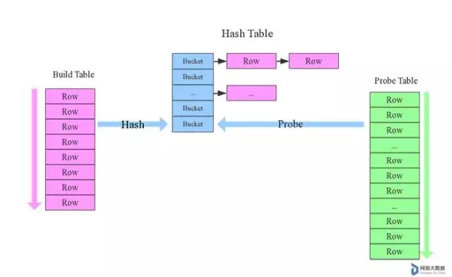
基本流程可以参考上图,这里有两个小问题需要关注:

  1. hash join性能如何?

很显然,hash join基本都只扫描两表一次,可以认为o(a+b),较之最极端的笛卡尔集运算a*b,效率大大提升。

  1. 为什么Build Table选择小表?

道理很简单,因为构建的Hash Table最好能全部加载在内存,效率最高;这也决定了hash join算法只适合至少一个小表的join场景,对于两个大表的join场景并不适用。

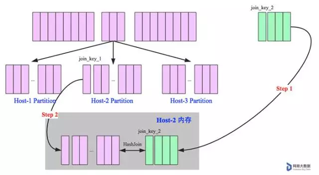
hash join是传统数据库中的单机join算法,在分布式环境下需要经过一定的分布式改造,就是尽可能利用分布式计算资源进行并行化计算,提高总体效率。hash join分布式改造一般有两种经典方案:

  1. broadcast hash join

将其中一张小表广播分发到另一张大表所在的分区节点上,分别并发地与其上的分区记录进行hash join。broadcast适用于小表很小,可以直接广播的场景。

  1. shuffled hash join

一旦小表数据量较大,此时就不再适合进行广播分发。这种情况下,可以根据join key相同必然分区相同的原理,将两张表分别按照join key进行重新组织分区,这样就可以将join分而治之,划分为很多小join,充分利用集群资源并行化。

下面分别进行详细讲解。

BroadcastHashJoinExec

  1. broadcast阶段:

将小表广播分发到大表所在的所有主机。广播算法可以有很多,最简单的是先发给driver,driver再统一分发给所有executor;要不就是基于BitTorrent的TorrentBroadcast。

  1. hash join阶段:

在每个executor上执行单机版hash join,小表映射,大表试探。

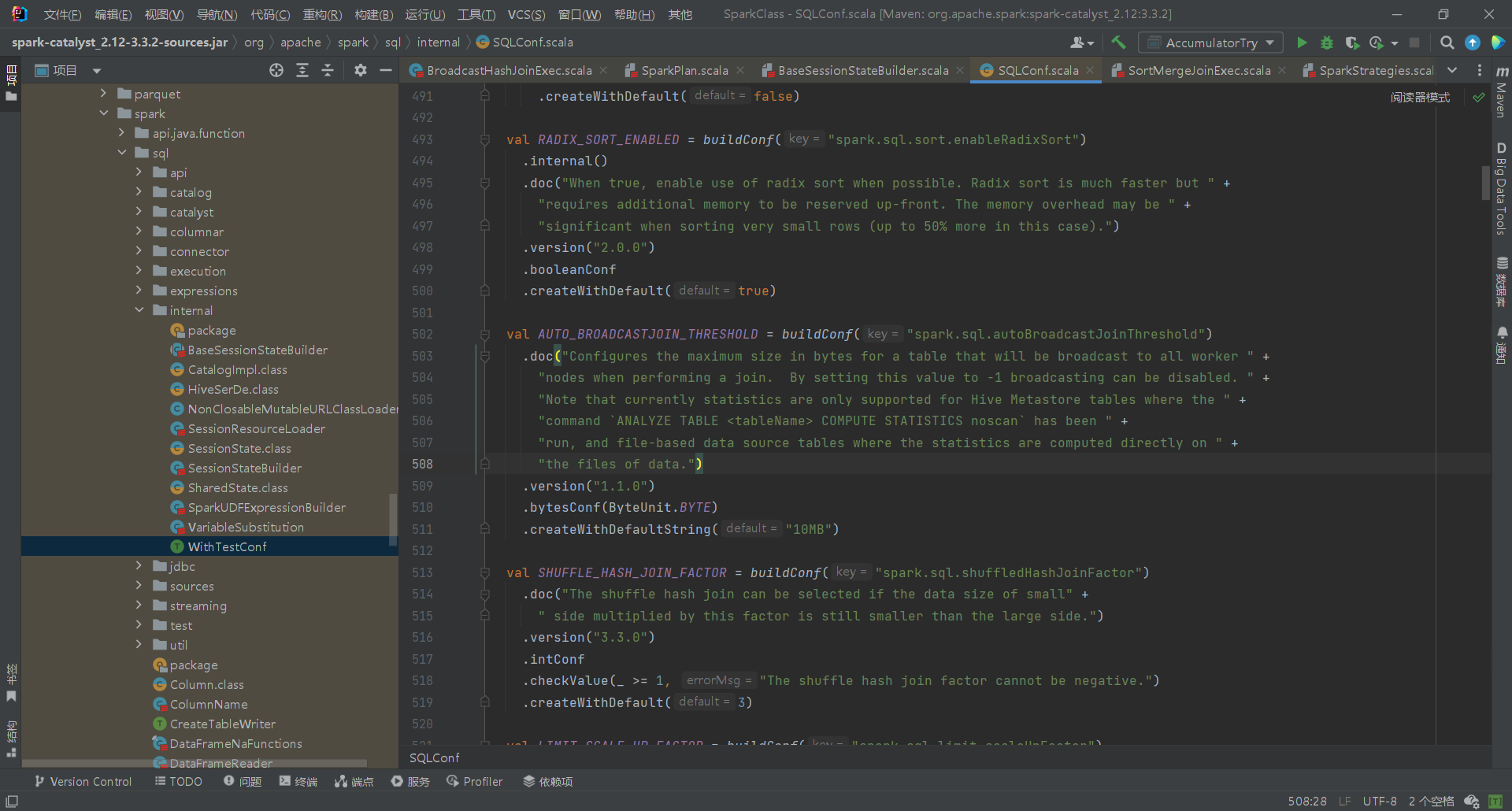
SparkSQL规定broadcast hash join执行的基本条件为被广播小表必须小于参数spark.sql.autoBroadcastJoinThreshold,默认为10M。 源码位于org.apache.spark.sql.internal.SQLConf.scala,没找到SQLConf文件可以在BaseSessionStateBuilder里找到conf引用,然后CTRL+左键查看源码。

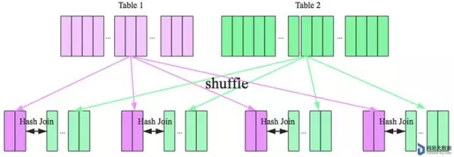
ShuffledHashJoinExec

在大数据条件下如果一张表很小,执行join操作最优的选择无疑是broadcast hash join,效率最高。但是一旦小表数据量增大,广播所需内存、带宽等资源必然就会太大,broadcast hash join就不再是最优方案。此时可以按照join key进行分区,根据key相同必然分区相同的原理,就可以将大表join分而治之,划分为很多小表的join,充分利用集群资源并行化。如下图所示,shuffle hash join也可以分为两步:

  1. shuffle阶段:

分别将两个表按照join key进行分区,将相同join key的记录重分布到同一节点,两张表的数据会被重分布到集群中所有节点。这个过程称为shuffle。

  1. hash join阶段:

每个分区节点上的数据单独执行单机hash join算法。

SortMergeJoinExec

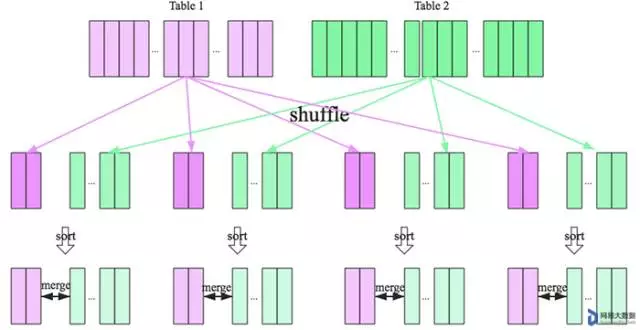
SparkSQL对两张大表join采用了全新的算法——sort merge join,整个过程分为三个步骤:

  1. shuffle阶段:

将两张大表根据join key进行重新分区,两张表数据会分布到整个集群,以便分布式并行处理。

  1. sort阶段:

对单个分区节点的两表数据,分别进行排序。

  1. merge阶段:

对排好序的两张分区表数据执行join操作。join操作很简单,分别遍历两个有序序列,碰到相同join key就merge输出,否则取更小一边。如下图所示:

CartesianProductExec:

  1. 初始化:两个数据集被加载并分区。
  2. 分区组合:每个分区的所有元素与另一个分区的所有元素组合。这在逻辑上类似于嵌套循环。
  3. 生成所有组合:对每一对元素生成一个元组,形成笛卡尔积。结果集的大小为两个数据集大小的乘积。

笛卡尔积会占用大量内存,使用笛卡尔积之前最好先过滤掉无用数据,其中一张表为极小表时建议广播。

BroadcastNestedLoopJoinExec

  1. broadcast阶段:将小表的数据复制并广播到大表分区数据所在的每个执行节点。
  2. 嵌套循环连接:
    • 在每个执行节点上,对于分区中的每一行,逐行扫描广播的小表。
    • 对每一对行执行连接条件,生成匹配的结果。
  3. 生成结果:将匹配的行组合成结果集。结果在每个节点独立生成,最后输出为完整的连接结果。

另外,Spark对非等值连接的支持只有这种和笛卡尔积(CartesianProduct)。 如果两张表都很大且无法广播,Spark 可能需要通过优化或变通的方法来处理:

  • 数据过滤:在连接前尽量过滤数据,减少处理的数据量。
  • 分区和缓存:有效地分区和缓存数据以提高性能。
  • 自定义 UDF:在某些情况下,使用自定义 UDF 可能会帮助实现复杂的连接逻辑。

选择join的机制

相关源码位于org.apache.spark.sql.execution下的141行JoinSelection对象

根据连接策略提示、等价连接键的可用性和连接关系的大小,选择合适的连接物理计划。 以下是现有的连接策略、其特点和局限性。

  • broadcast hash join(BHJ): 仅支持等价连接,而连接键无需可排序。 支持除全外部连接外的所有连接类型。 当广播方较小时,BHJ 通常比其他连接算法执行得更快。 不过,广播表是一种网络密集型操作,在某些情况下可能会导致 OOM 或性能不佳,尤其是当构建/广播方较大时。
  • shuffled hash join: 仅支持等价连接,而连接键无需可排序。 支持所有连接类型。 从表中构建哈希映射是一个内存密集型操作,当联编侧很大时可能会导致 OOM。
  • shuffle sort merge join(SMJ): 仅支持等连接,且连接键必须是可排序的。 支持所有连接类型。
  • Broadcast nested loop join(广播嵌套循环连接 BNLJ): 支持等连接和非等连接。 支持所有连接类型,但优化了以下方面的实现: 1)在右外连接中广播左侧;2)在左外、左半、左反或存在连接中广播右侧;3)在类内连接中广播任一侧。 对于其他情况,我们需要多次扫描数据,这可能会相当慢。
  • Shuffle-and-replicate nested loop join (洗牌复制嵌套循环连接,又称笛卡尔积连接): 支持等连接和非等连接。 只支持内同类连接。

源码中关于等值连接选择join的机制介绍如下:

 1
 2
 3
 4
 5
 6
 7
 8
 9
10
11
12
13
14
15
16
17
18
19
If it is an equi-join, we first look at the join hints w.r.t. the following order:
   1. broadcast hint: pick broadcast hash join if the join type is supported. If both sides
      have the broadcast hints, choose the smaller side (based on stats) to broadcast.
   2. sort merge hint: pick sort merge join if join keys are sortable.
   3. shuffle hash hint: We pick shuffle hash join if the join type is supported. If both
      sides have the shuffle hash hints, choose the smaller side (based on stats) as the
      build side.
   4. shuffle replicate NL hint: pick cartesian product if join type is inner like.

 If there is no hint or the hints are not applicable, we follow these rules one by one:
   1. Pick broadcast hash join if one side is small enough to broadcast, and the join type
      is supported. If both sides are small, choose the smaller side (based on stats)
      to broadcast.
   2. Pick shuffle hash join if one side is small enough to build local hash map, and is
      much smaller than the other side, and `spark.sql.join.preferSortMergeJoin` is false.
   3. Pick sort merge join if the join keys are sortable.
   4. Pick cartesian product if join type is inner like.
   5. Pick broadcast nested loop join as the final solution. It may OOM but we don't have
      other choice.

翻译如下:

如果是等值连接,我们首先按以下顺序查看连接提示(join hints):

  1. broadcast hint:如果支持广播散列连接(BHJ),则选择广播散列连接。 如果双方有广播提示,则选择较小的一方(根据统计信息)进行广播。
  2. sort merge hint:如果连接键可排序,则选择排序合并连接。
  3. shuffle hash hint:如果支持连接类型,我们会选择洗牌散列连接。 如果双方都有洗牌散列提示,则选择较小的一方(基于统计信息)作为构建方。 构建侧。
  4. shuffle replicate NL 提示:如果连接类型是内连接,则选择笛卡尔积。

如果没有提示或提示不适用,我们将逐一遵循这些规则:

  1. 如果有一方足够小,可以广播,且连接类型支持,则选择广播散列连接。 支持。 如果两边都很小,则选择较小的一边(根据统计数据) 进行广播。
  2. 如果一方的规模小到足以建立本地哈希映射,并且比另一方小很多,并且支持 “space”,则选择 “洗牌哈希连接”。 且 spark.sql.join.preferSortMergeJoin 为 false。
  3. 如果连接键可排序,则选择排序合并连接。
  4. 如果连接类型为inner join(就是不明写join的join,即类似select * from order,item),则选择笛卡尔积。
  5. 选择广播嵌套循环连接作为最终解决方案。 可能会出现 OOM,但我们没有 其他选择。

相关关键源码如下:

 1
 2
 3
 4
 5
 6
 7
 8
 9
10
11
12
13
14
15
16
17
18
19
20
21
22
def createJoinWithoutHint() = {
  createBroadcastHashJoin(false)
    .orElse(createShuffleHashJoin(false))
    .orElse(createSortMergeJoin())
    .orElse(createCartesianProduct())
    .getOrElse {
      // This join could be very slow or OOM
      val buildSide = getSmallerSide(left, right)
      Seq(joins.BroadcastNestedLoopJoinExec(
        planLater(left), planLater(right), buildSide, joinType, j.condition))
    }
}
        
if (hint.isEmpty) {
  createJoinWithoutHint()
} else {
  createBroadcastHashJoin(true)
    .orElse { if (hintToSortMergeJoin(hint)) createSortMergeJoin() else None }
    .orElse(createShuffleHashJoin(true))
    .orElse { if (hintToShuffleReplicateNL(hint)) createCartesianProduct() else None }
    .getOrElse(createJoinWithoutHint())
}

综上所述:

  1. 有连接提示时,优先级从高到低:BroadcastHashJoin > SortMergeJoin > ShuffledHashJoin > CartesianProduct
  2. 没有连接提示时,优先级从高到低(join代价从小到大):BroadcastHashJoin > ShuffledHashJoin > SortMergeJoin > CartesianProduct > BroadcastNestedLoopJoin

注意:有提示时优先SortMergeJoin,然后ShuffledHashJoin;而没有提示时,优先ShuffledHashJoin,然后SortMergeJoin

总结: 数据仓库设计时最好避免大表与大表的join查询,SparkSQL也可以根据内存资源、带宽资源适量将参数spark.sql.autoBroadcastJoinThreshold调大,让更多join实际执行为broadcast hash join。

  1. 大表join极小表(表大小小于10M,可调整spark.sql.autoBroadcastJoinThreshold参数进行修改),用BroadcastHashJoin
  2. 大表join小表,用ShuffledHashJoin
  3. 大表join大表,用SortMergeJoin

非等值连接仅CartesianProduct 和 BroadcastNestedLoopJoin支持,常用BroadcastNestedLoopJoin。

补充:RDD中的join

前文中介绍的join都是SparkSQL中join的底层实现,但是在Spark的RDD中,也有一个join函数。 具体实现如下:

 1
 2
 3
 4
 5
 6
 7
 8
 9
10
11
12
13
14
15
16
17
18
19
20
21
22
23
24
25
26
27
28
29
30
31
32
33
34
35
36
37
38
39
40
41
42
43
44
45
46
47
48
49
50
51
52
53
54
55
56
57
58
59
60
61
62
  /**
   * Return an RDD containing all pairs of elements with matching keys in `this` and `other`. Each
   * pair of elements will be returned as a (k, (v1, v2)) tuple, where (k, v1) is in `this` and
   * (k, v2) is in `other`. Uses the given Partitioner to partition the output RDD.
   */
  def join[W](other: RDD[(K, W)], partitioner: Partitioner): RDD[(K, (V, W))] = self.withScope {
    this.cogroup(other, partitioner).flatMapValues( pair =>
      for (v <- pair._1.iterator; w <- pair._2.iterator) yield (v, w)
    )
  }

  /**
   * Perform a left outer join of `this` and `other`. For each element (k, v) in `this`, the
   * resulting RDD will either contain all pairs (k, (v, Some(w))) for w in `other`, or the
   * pair (k, (v, None)) if no elements in `other` have key k. Uses the given Partitioner to
   * partition the output RDD.
   */
  def leftOuterJoin[W](
      other: RDD[(K, W)],
      partitioner: Partitioner): RDD[(K, (V, Option[W]))] = self.withScope {
    this.cogroup(other, partitioner).flatMapValues { pair =>
      if (pair._2.isEmpty) {
        pair._1.iterator.map(v => (v, None))
      } else {
        for (v <- pair._1.iterator; w <- pair._2.iterator) yield (v, Some(w))
      }
    }
  }

  /**
   * Perform a right outer join of `this` and `other`. For each element (k, w) in `other`, the
   * resulting RDD will either contain all pairs (k, (Some(v), w)) for v in `this`, or the
   * pair (k, (None, w)) if no elements in `this` have key k. Uses the given Partitioner to
   * partition the output RDD.
   */
  def rightOuterJoin[W](other: RDD[(K, W)], partitioner: Partitioner)
      : RDD[(K, (Option[V], W))] = self.withScope {
    this.cogroup(other, partitioner).flatMapValues { pair =>
      if (pair._1.isEmpty) {
        pair._2.iterator.map(w => (None, w))
      } else {
        for (v <- pair._1.iterator; w <- pair._2.iterator) yield (Some(v), w)
      }
    }
  }

  /**
   * Perform a full outer join of `this` and `other`. For each element (k, v) in `this`, the
   * resulting RDD will either contain all pairs (k, (Some(v), Some(w))) for w in `other`, or
   * the pair (k, (Some(v), None)) if no elements in `other` have key k. Similarly, for each
   * element (k, w) in `other`, the resulting RDD will either contain all pairs
   * (k, (Some(v), Some(w))) for v in `this`, or the pair (k, (None, Some(w))) if no elements
   * in `this` have key k. Uses the given Partitioner to partition the output RDD.
   */
  def fullOuterJoin[W](other: RDD[(K, W)], partitioner: Partitioner)
      : RDD[(K, (Option[V], Option[W]))] = self.withScope {
    this.cogroup(other, partitioner).flatMapValues {
      case (vs, Seq()) => vs.iterator.map(v => (Some(v), None))
      case (Seq(), ws) => ws.iterator.map(w => (None, Some(w)))
      case (vs, ws) => for (v <- vs.iterator; w <- ws.iterator) yield (Some(v), Some(w))
    }
  }

RDD的join实际是匹配两个RDD,以join为例,遍历(iterator)两个RDD的分区,调用cogroup函数将两个RDD的相同分区联合成一个turple返回。

页面浏览量Loading
网站总访客数:Loading
网站总访问量:Loading
使用 Hugo 构建
主题 StackJimmy 设计